Training intelligent adversaries using self-play with ML-Agents


In the latest release of the ML-Agents Toolkit (v0.14), we have added a self-play feature that provides the capability to train competitive agents in adversarial games (as in zero-sum games, where one agent’s gain is exactly the other agent’s loss). In this blog post, we provide an overview of self-play and demonstrate how it enables stable and effective training on the Soccer demo environment in the ML-Agents Toolkit.
The Tennis and Soccer example environments of the Unity ML-Agents Toolkit pit agents against one another as adversaries. Training agents in this type of adversarial scenario can be quite challenging. In fact, in previous releases of the ML-Agents Toolkit, reliably training agents in these environments required significant reward engineering. In version 0.14, we have enabled users to train agents in games via reinforcement learning (RL) from self-play, a mechanism fundamental to a number of the most high profile results in RL such as OpenAI Five and DeepMind’s AlphaStar. Self-play uses the agent’s current and past ‘selves’ as opponents. This provides a naturally improving adversary against which our agent can gradually improve using traditional RL algorithms. The fully trained agent can be used as competition for advanced human players.
Self-play provides a learning environment analogous to how humans structure competition. For example, a human learning to play tennis would train against opponents of similar skill level because an opponent that is too strong or too weak is not as conducive to learning the game. From the standpoint of improving one’s skills, it would be far more valuable for a beginner-level tennis player to compete against other beginners than, say, against a newborn child or Novak Djokovic. The former couldn’t return the ball, and the latter wouldn’t serve them a ball they could return. When the beginner has achieved sufficient strength, they move on to the next tier of tournament play to compete with stronger opponents.
In this blog post, we give some technical insight into the dynamics of self-play as well as provide an overview of our Tennis and Soccer example environments that have been refactored to showcase self-play.
History of self-play in games
The notion of self-play has a long history in the practice of building artificial agents to solve and compete with humans in games. One of the earliest uses of this mechanism was Arthur Samuel’s checker playing system, which was developed in the ’50s and published in 1959. This system was a precursor to the seminal result in RL, Gerald Tesauro’s TD-Gammon published in 1995. TD-Gammon used the temporal difference learning algorithm TD(λ) with self-play to train a backgammon agent that nearly rivaled human experts. In some cases, it was observed that TD-Gammon had a superior positional understanding to world-class players.
Self-play has been instrumental in a number of contemporary landmark results in RL. Notably, it facilitated the learning of super-human Chess and Go agents, elite DOTA 2 agents, as well as complex strategies and counter strategies in games like wrestling and hide and seek. In results using self-play, the researchers often point out that the agents discover strategies which surprise human experts.
Self-play in games imbues agents with a certain creativity, independent of that of the programmers. The agent is given just the rules of the game and told when it wins or loses. From these first principles, it is up to the agent to discover competent behavior. In the words of the creator of TD-Gammon, this framework for learning is liberating “...in the sense that the program is not hindered by human biases or prejudices that may be erroneous or unreliable.” This freedom has led agents to uncover brilliant strategies that have changed the way human experts view certain games.
Reinforcement Learning in adversarial games
In a traditional RL problem, an agent tries to learn a behavior policy that maximizes some accumulated reward. The reward signal encodes an agent’s task, such as navigating to a goal state or collecting items. The agent’s behavior is subject to the constraints of the environment. For example, gravity, the presence of obstacles, and the relative influence the agent’s own actions have, such as applying force to move itself are all environmental constraints. These limit the viable agent behaviors and are the environmental forces the agent must learn to deal with to obtain a high reward. That is, the agent contends with the dynamics of the environment so that it may visit the most rewarding sequences of states.

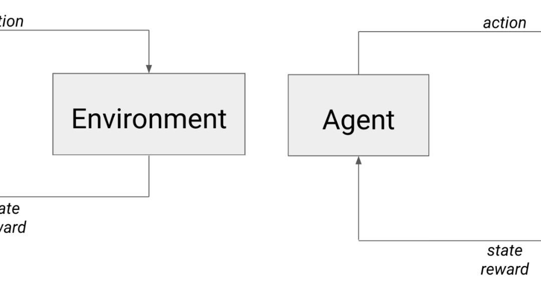
On the left is the typical RL scenario: an agent acts in the environment and receives the next state and a reward On the right is the learning scenario wherein the agent competes with an adversary who, from the agent’s perspective, is effectively part of the environment.
In the case of adversarial games, the agent contends not only with the environment dynamics, but also another (possibly intelligent) agent. You can think of the adversary as being embedded in the environment since its actions directly influence the next state the agent observes as well as the reward it receives.

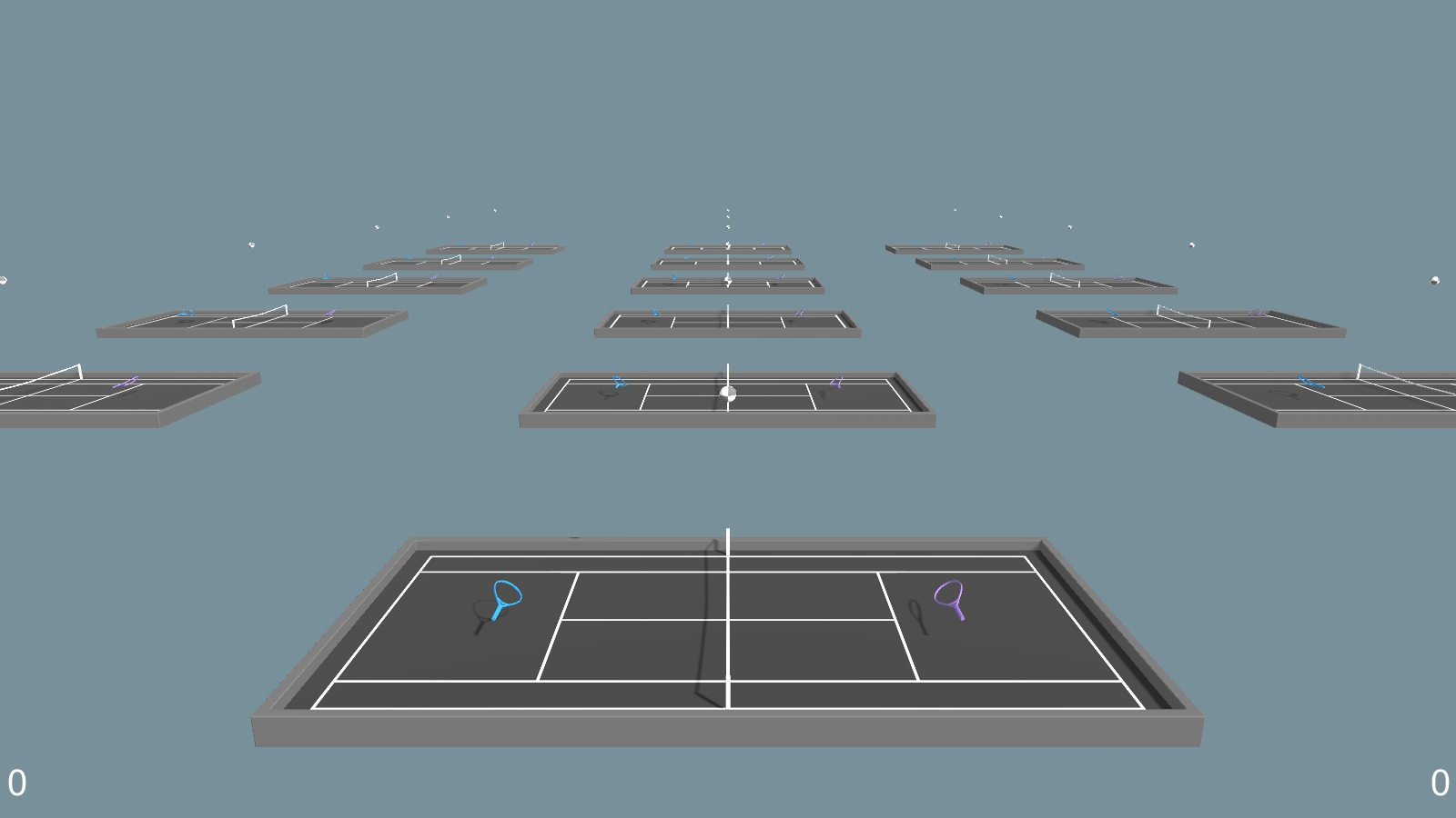
The Tennis example environment from the ML-Agents Toolkit
Let’s consider the ML-Agents Tennis demo. The blue racquet (left) is the learning agent, and the purple racquet (right) is the adversary. To hit the ball over the net, the agent must consider the trajectory of the incoming ball and adjust it’s angle and speed accordingly to contend with gravity (the environment). However, just getting the ball over the net is only half the battle when there is an adversary. A strong adversary may return a winning shot causing the agent to lose. A weak adversary may hit the ball into the net. An equal adversary may return the ball, thereby continuing the game. In any case, the next state and reward are determined by both the environment and the adversary. However, in all three situations, the agent hit the same shot. This makes learning in adversarial games and training competitive agent behaviors a difficult problem.
The considerations around an appropriate opponent are not trivial. As demonstrated by the preceding discussion, the relative strength of the opponent has a significant impact on the outcome of an individual game. If an opponent is too strong, it may be too difficult for an agent starting from scratch to improve. On the other hand, if an opponent is too weak, an agent may learn to win, but the learned behavior may not be useful against a different or stronger opponent. Therefore, we need an opponent that is roughly equal in skill (challenging but not too challenging). Additionally, since our agent is improving with each new game, we need an equivalent increase in the opponent.


In self-play, a past snapshot or the current agent is the adversary embedded in the environment.
Self-play to the rescue! The agent itself satisfies both requirements for a fitting opponent. It is certainly roughly equal in skill (to itself) and also improves over time. In this case, it is the agent’s own policy that is embedded in the environment (see figure). For those familiar with curriculum learning, you can think of this as a naturally evolving (also referred to as an auto-curricula) curriculum for training our agent against opponents of increasing strength. Thus, self-play allows us to bootstrap an environment to train competitive agents for adversarial games!
In the following two subsections, we consider more technical aspects of training competitive agents, as well as some details surrounding the usage and implementation of self-play in the ML-Agents Toolkit. These two subsections may be skipped without loss to the main point of this blog post.
Practical considerations
Some practical issues arise from the self-play framework. Specifically, overfitting to defeat a particular playstyle and instability in the training process that can arise from non-stationarity of the transition function (i.e., the constantly shifting opponent). The former is an issue because we want our agents to be general competitors and robust to different types of opponents. To illustrate the latter, in the Tennis environment, a different opponent will return the ball at a different angle and speed. From the perspective of the learning agent, this means the same decisions will lead to different next states as training progresses. Traditional RL algorithms assume stationary transition functions. Unfortunately, by supplying the agent with a diverse set of opponents to address the former, we may exacerbate the latter if we are not careful.
To address this, we maintain a buffer of the agent’s past policies from which we sample opponents against which the learner competes for a longer duration. By sampling from the agent’s past policies, the agent will see a diverse set of opponents. Furthermore, letting the agent train against a fixed opponent for a longer duration stabilizes the transition function and creates a more consistent learning environment. Additionally, these algorithmic aspects can be managed with the hyperparameters discussed in the next section.
Implementation and usage details
With self-play hyperparameter selection, the main consideration is the tradeoff between the skill level and generality of the final policy, and the stability of learning. Training against a set of slowly changing or unchanging adversaries with low diversity results in a more stable learning process than training against a set of quickly changing adversaries with high diversity. The available hyperparameters control how often an agent’s current policy is saved to be used later as a sampled adversary, how often a new adversary is sampled, the number of opponents saved, and the probability of playing against the agent’s current self versus an opponent sampled from the pool. For usage guidelines of the available self-play hyperparameters, please see the self-play documentation in the ML-Agents GitHub repository.
In adversarial games, the cumulative environment reward may not be a meaningful metric by which to track learning progress. This is because the cumulative reward is entirely dependent on the skill of the opponent. An agent at a particular skill level will get more or less reward against a worse or better agent, respectively. We provide an implementation of the ELO rating system, a method for calculating the relative skill level between two players from a given population in a zero-sum game. In a given training run, this value should steadily increase. You can track this using TensorBoard along with other training metrics e.g. cumulative reward.
Self-play and Soccer Environment


In recent releases, we have not included an agent policy for our Soccer example environment because it could not be reliably trained. However, with self-play and some refactoring, we are now able to train non-trivial agent behaviors. The most significant change is the removal of “player positions” from the agents. Previously, there was an explicit goalie and striker, which we used to make the gameplay look reasonable. In the video below of the new environment, we actually notice role-like, cooperative behavior along these same lines of goalie and striker emerge. Now the agents learn to play these positions on their own! The reward function for all four agents is defined as +1.0 for scoring a goal and -1.0 for getting scored on with an additional per-timestep penalty of -0.0003 to encourage agents to score.
We emphasize the point that training agents in the Soccer environment led to cooperative behavior without an explicit multi-agent algorithm or assigning roles. This result shows that we can train complicated agent behaviors with simple algorithms as long as we take care in formulating our problem. The key to achieving this is that agents can observe their teammates---that is, agents receive information about their teammate’s relative position as observations. By making an aggressive play toward the ball, the agent implicitly communicates to its teammate that it should drop back on defense. Alternatively, by dropping back on defense, it signals to its teammate that it can move forward on offense. The video above shows the agents picking up on these cues as well as demonstrating general offensive and defensive positioning!
The self-play feature will enable you to train new and interesting adversarial behaviors in your game. If you do use the self-play feature, please let us know how it goes!
Next steps
If you’d like to work on this exciting intersection of machine learning and games, we are hiring for several positions, please apply!
If you use any of the features provided in this release, we’d love to hear from you. For any feedback regarding the Unity ML-Agents Toolkit, please fill out the following survey and feel free to email us directly. If you encounter any bugs, please reach out to us on the ML-Agents GitHub issues page. For any general issues and questions, please reach out to us on the Unity ML-Agents forums.
Is this article helpful for you?
Thank you for your feedback!
- Unity Labs
- Copyright © 2024 Unity Technologies